ORBS Reduction Guide (Outdated)¶

Contents

ORBS Reduction Guide (Outdated)

A 2 steps reduction ¶

Each reduction can be divided in two major steps :

Creation of the option file
Start of the reduction process

The creation of the option file is certainly the most important step as this file contains all the parameters which will be passed to ORBS. Indeed this file controls all the important aspects of the reduction. While starting the reduction process can be reduced to typing a simple command line.

Creation of the option file ¶

Many parameters must be passed to ORBS for a reduction. An option file is just a list of these parameters recorded into a text file, each line being made of a keyword and its value, e.g.:

OBJECT M1-67 # Object name
FILTER SPIOMM_R # Filter
SPESTEP 3852 # Step size in nm
SPESTNB 415 # Step nb
SPEORDR 11 # Aliasing order
SPEEXPT 30 # Integration time
DIRCAM1 /data/spiomm/M1-67/cam1/ # Path to the raw images of the camera 1
DIRCAM2 /data/spiomm/M1-67/cam2/ # Path to the raw images of the camera 2
DIRCAL1 /data/spiomm/M1-67/HeNe/ # Calibration laser images of camera 1

Some of the parameters in this file must be present while some are just optional.

Required parameters ¶

The following parameters are required if you want to transform you raw interferometric images into a spectral cube:

OBJECT: The name of the object. It is only used to name the output files and can be anything (as long as it does not contain any white space).
FILTER: Must be a valid name. The list of the available filters can be found in ORB data folder (orb/data/filter_*). For SITELLE’s data you can refer to the keyword FILTER in the header of the data files.
SPESTEP: Step size in nm. At this point it is not directly given in the header of SITELLE’s data and must be calculated (see How to compute the step size in nm from SITELLE’S data files header ?).
SPESTNB: Number of steps expected in the scan (i.e. number of raw files acquired if the scan has been completed). It must be at least equal to the number of raw images.
SPEORDR: Aliasing (or folding) order (you can refer to SITORDER in SITELLE’s files header).
DIRCAM1: Absolute path to the raw images of the camera 1
DIRCAM2: Absolute path to the raw images of the camera 2 (For SITELLE both paths must be the same)
SPEEXPT: Integration time of each frame (in s)
DIRCAL1: Path to the folder containing the calibration laser images of the camera 1.

Note

When a path to a folder is expected, the folder must only contain the requested files (i.e. the folder set to DIRCAL1 must only contain the images of the calibration laser cube). Note also that only FITS files will be considered, i.e. you can put any other type of file in this folder. If all you FITS files must be in the same folder you can give the path to a file list (see File list) in place of a path to a folder.

How to compute the step size in nm from SITELLE’S data files header ?¶

The following formula can be used:

\[\frac{(n + 1) \times \lambda_{\text{min}}}{2}\]

\(n\) : Aliasing order (SITORDER)

\(\lambda_{\text{min}}\) : Minimum wavelength of the filter (SITLAMIN)

Optional parameters ¶

The following parameters are considered as optional because you can get a spectral cube without them. But they might prove useful if you want to correct your images for the bias, dark current and flat field and calibrate your files in energy, angle and wavelength.

Bias, dark and flat field correction ¶

DIRBIA1: Path to a folder containing the bias frames of the camera 1.
DIRBIA2: Path to a folder containing the bias frames of the camera 2.
DIRDRK1: Path to a folder containing the dark frames of the camera 1.
DIRDRK2: Path to a folder containing the dark frames of the camera 2.
DIRFLT1: Path to a folder containing the flat frames of the camera 1.
DIRFLT2: Path to a folder containing the flat frames of the camera 2.

DIRBIA1 /home/thomas/Réduction/Données/Data_2012_06/BIAS/cam1
DIRBIA2 /home/thomas/Réduction/Données/Data_2012_06/BIAS/cam2/4x4
DIRDRK1 /home/thomas/Réduction/Données/Data_2012_06/DARK/cam1
DIRDRK2 /home/thomas/Réduction/Données/Data_2012_06/DARK/cam2/4x4
DIRFLT1 /home/thomas/Réduction/Données/Data_2012_06/FLAT/R/cam1/3x3
DIRFLT2 /home/thomas/Réduction/Données/Data_2012_06/FLAT/R/cam2/4x4

Warning

SITELLE: Bias correction is automatically done from the overscan part of the data: do not give a path to bias frames because it will result in subtracting two times the bias.

Warning

SpIOMM: In the recent observations, a bias frame is taken at each exposition with the camera 2. In this case the bias is automatically subtracted. Only the path to the bias files for the camera 1 is thus required. Giving a path for the bias frames of the camera 2 would result in subtracting two times the bias.

Calibration data ¶

CALIBMAP: Path to a calibration laser map. The way you can obtain this map is described at the section Laser cube (wavelength/wavenumber calibration). If the same calibration laser cube is used for multiple science cubes it is faster to compute the calibration map once and for all instead.
STDPATH: Path to the spectrum of a standard star. The spectrum must have been reduced by ORBS following the procedure described at the section Standard star (photometrical calibration). STDNAME must also be set.
STDNAME: Name of the standard star. A list of the available standard name can be found in ORB data folder: orb/data/std_table.orb:
```
STDNAME HD74721
STDPATH /data/calib/HD74721/HD74721_SPIOMM_R.merged.standard_spectrum.fits
```
TARGETX, TARGETY, TARGETR, TARGETD: Image position along X and Y axis and celestial coordinates (RA, DEC) of a point near the center of the image. The astrometrical calibration will be computed from a star catalog query (USNO-B1) around this point (An internet connection must be available):
```
TARGETR 19:11:30.857
TARGETD +16:51:39.92
TARGETX 214.31944
TARGETY 205.87269
```
PHAPATH: Path to the phase map created from a continuum source cube (see Continuum source cube (Phase map))

Start of the reduction process ¶

Start command ¶

The reduction process can be started with the command (see How can I have access to ORBS commands ?):

orbs options.opt start

At the end of the process the reduced cube is written in the root folder where you have launched the command, e.g. M1-67_SPIOMM_R.merged.nm.1.0.fits. Its exact name can change depending on the kind of chosen output (see Choosing the right output).

Note

It is recommended that you create a new folder where you can put your option file (e.g. options.opt) and start the reduction process.

Choosing your starting step ¶

Sometimes it can be useful to restart a reduction from a particular step in order to change the reduction output type (or because of an error, but in this case, the resume operation is generally better see Other operations with orbs command). This can be achieved with the option --step followed by the step number, e.g.:

orbs options.opt start --step 11

The step number changes with the desired target (see Reduce your calibration files). For the default target (an astrophysical object) the Road Map is:

Compute alignment vector (camera 1).
Compute alignment vector (camera 2).
Compute cosmic ray map (camera 1)
Compute cosmic ray map (camera 2)
Compute interferogram (camera 1)
Compute interferogram (camera 2)
Transform cube B
Merge interferograms
Compute calibration laser map (camera 1)
Compute phase
Compute phase maps
Compute spectrum
Calibrate spectrum

Note

When typing orbs options.opt start -h you can get the roadmaps of some targets.

Other operations with orbs command ¶

Other operations are possible with the orbs command:

resume: Resume the last reduction process launched. If all the steps have been done, the output file is written again on the root folder:

orbs options.opt resume

clean: Clean the directory from the files created during the reduction:

orbs options.opt clean

status: Display the status (Road Map and step status) of all the launched reduction processes:

orbs options.opt status

Note

All the operations are attached to the option file of the command line.

Reduction files ¶

A lot of reduction files are created during the process. The most important are described here.

Temporary reduction folder ¶

First of all a temporary reduction folder is created. It is named after the object name and the filter used (e.g. M1-67_SPIOMM_R/). This way different data cubes of the same object taken with different filters can be reduced in the same folder.

Log file ¶

A log file named after the option file (e.g. options.opt.log) is created. It contains all the comments, warnings and error messages that are displayed on the screen.

Reduce your calibration files ¶

Laser cube (wavelength/wavenumber calibration)¶

The wavelength calibration is certainly the most important one for its difficulty to be achieved independently on the spectral cube itself. This calibration is also necessary to get a cube for eye-checking purpose (see Why you might not want the spectral calibration).

A laser cube at a calibrated wavelength must be reduced to obtain a calibration map. A calibration map gives the measured wavelength of the laser for each pixel of the image.

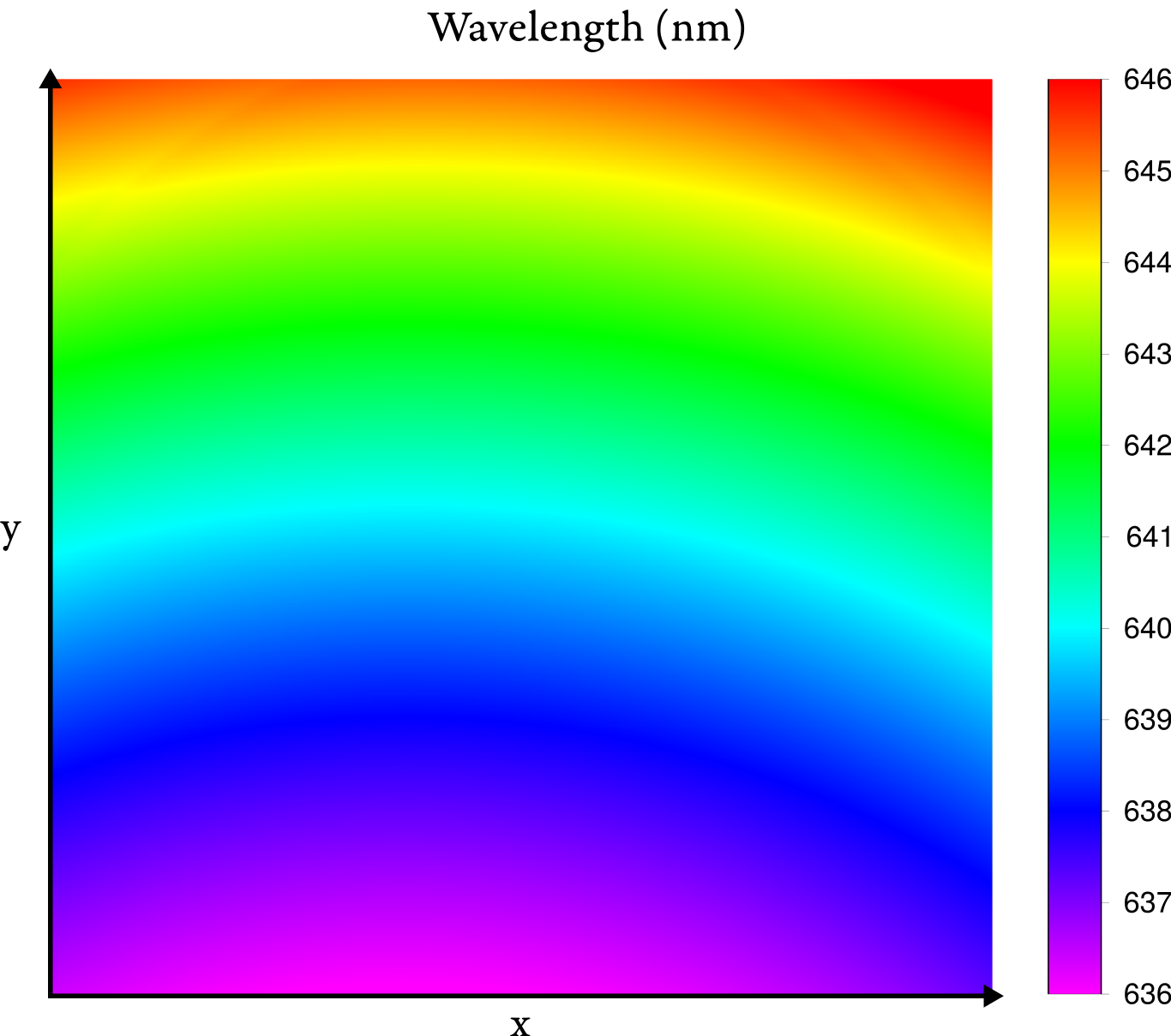
The above figure shows a typical calibration map of SpIOMM (The measured wavelength is given in nm).

Option file ¶

If the laser cube has been taken with the default observation parameters (step, order – those parameters are defined in the ORB configuration file) the only required keyword is DIRCAL1:

## Laser configuration file
DIRCAL1 /path/to/the/calibration/laser/folder # Path to the calibration laser folder

If the observation parameters are not the default ones the keywords SPESTEP and SPEORDR have to be added:

## Laser configuration file

DIRCAL1 /path/to/the/calibration/laser/folder # Path to the calibration laser folder
SPESTEP 9765 # Step size (in nm)
SPEORDR 30 # Aliasing order

Reduction command ¶

The reduction command is simply:

orbs laser.opt start --laser

Output file ¶

The output file is a calibration laser map named LASER_None.cam1.calibration_laser_map.fits

Standard star (photometrical calibration)¶

Reducing a standard star is nearly equivalent to the reduction of another astrophysical object. The only difference is the output file which is not a spectral cube but a single spectrum.

Option file ¶

The required keywords are the same as defined at the section Required parameters except that the two keywords TARGETX and TARGETY giving the position of the standard star in the image are also required. A minimal option file would be, e.g.:

OBJECT HD74721 # Object name
FILTER SPIOMM_R # Filter name
SPESTEP 4180 # Step size (in nm)
SPESTNB 377 # Number of steps
SPEORDR 12 # Aliasing order
SPEEXPT 3 # Integration time
TARGETX 223 # X position of the standard
TARGETY 268 # Y position of the standard
DIRCAM1 /path/to/standard/folder/HD74721/R # Standard CAM1 folder path
DIRCAM2 /path/to/standard/folder/HD74721/R/CAM2 # Standard CAM2 folder path
DIRCAL1 /path/to/calibration/folder/HeNe # Path to the calibration laser cube folder

Note

The position has not to be more precise than 1 pixel.

Warning

Indexing in ds9 starts with 1 while it starts with 0 in python so don’t forget to subtract 1 to the position read in ds9.

Reduction command ¶

The reduction command is:

orbs standard.opt start --standard

Output file ¶

The output file is a single spectrum in FITS format. With the example option file above it would be HD74721_SPIOMM_R.merged.standard_spectrum.fits.

Continuum source cube (Phase map)¶

A continuum source cube (e.g. a flat field observation) is used to compute a precise phase map (Up to now only SpIOMM is known to need a phase map).

It is characterized by the lack of star (or point) sources: no alignment can be done nor can the transmission vector be computed. So that all the star-dependant processes must be passed.

Option file ¶

The option file is exactly the same as an astronomical cube (see the section Required parameters). Only the command line call must be changed.

Reduction command ¶

The reduction command is:

orbs standard.opt start --flat

Output file ¶

The output file is a phase map in FITS format. Its name is e.g. CONTINNUM_SPIOMM_R.merged.flat_phase_map.fits.

It can be added to the astronomical object option file with the keyword PHAPATH.

Choosing the right output ¶

ORBS gives different possibilities for the output format of the spectral cube:

Spectral axis in wavelength (nm) or in wavenumber (\(\text{cm}^{-1}\)) (see Wavelength or wavenumber ?).
Apodization factor (see To apodize or not to apodize ?).
Spectral calibration or not (see Why you might not want the spectral calibration).

Choosing one option or the other depend on the use of the spectral cube. If you want to know quickly what are the best options for you, jump to the section Summary.

Wavelength or wavenumber ?¶

An interferogram is related to a spectrum by the Fourier Transform. The output of a Fourier Transform is a spectrum projected along an axis in wavenumber. One can pass from wavenumber to wavelength using:

\[\lambda [\text{nm}] = \frac{10^7}{\sigma [\text{cm}^{-1}]}\]

You immediately see where the problem: if the wavenumber axis is regular then the wavelength axis is not made of regularly spaced samples. The projection of the spectrum obtained directly after the FFT onto a regularly sampled wavelength axis relies on the interpolation of the spectrum: i.e. the spectral information is changed in an unpredictable way. Even if no error is made during the interpolation this also result in the deformation of the spectral line shape from a symmetrical gaussian or sinc line to an asymmetrical line.

You will thus have difficulties to fit a model (gaussian or sinc) on your spectral lines and the computed noise will be overestimated (SNR underestimated).

The only good news is that you will feel more comfortable with spectra projected onto a wavelength axis.

In summary:

If you just want to check your data: use a wavelength output
If you want to fit your data (or if you plan to use ORCS): you can use the wavenumber output.

To apodize or not to apodize ?¶

The spectral line shape of an unapodized spectrum is a sinc:

\[\text{sinc}(x) = \frac{\sin(x)}{x}\]

Some people doesn’t like it and prefer a Gaussian line shape. This is where the apodization becomes useful.

The apodization consists in multiplying the interferogram by a window with smooth edges (see e.g. Naylor 2007). The Fourier transform of the interferogram is thus convoluted to the Fourier transform of the window function, changing the original line shape (a sinc) to a more Gaussian-like shape.

The apodization factor in ORBS can be set to 1.0 (no apodization: sinc), 1.1, 1.2, 1.3, 1.4, 1.5, 1.6, 1.7, 1.8, 1.9, 2.0 (strongest apodization: gaussian).

In our case, as long as the user has the right model to fit its data the apodization is a transparent operation for everything (flux, velocity, amplitude) but the spectral resolution (fwhm) which is traded for a smoother line shape.

One problem is to fit the right model. With an apodization factor of 1.0 (no apodization) the model is a pure sinc. With an apodization of 2.0 (strongest apodization) the model is nearly a pure Gaussian. In between, the model is a mix of both functions without any known mathematical formulation. Don’t forget also that there is no good model if the axis is in wavelength because the lines are asymmetrical (see Wavelength or wavenumber ?)

The other problem is the loss of spectral resolution. The maximum spectral resolution is simply divided by the apodization factor.

In summary:

If you don’t care about the spectral resolution and are used to fitting Gaussian : use the 2.0 apodization function.
If you care about the spectral resolution and feel ready to fit sinc functions (or if you plan to use ORCS): use the 1.0 apodization function.

Why you might not want the spectral calibration ¶

In order to adjust all the spectra so that the samples with the same wavelength/wavenumber fall in the same channel, the spectral cube must be calibrated in wavelength/wavenumber (note that this calibration does not ensures that the wavelength/wavenumber corresponding to one channel is the exact one, you might better use a sky line for that purpose). But this operation makes use of interpolation which might change the spectral information in an unpredictable way.

If you want to have the purest spectra: just don’t ask for spectral calibration and use the calibration map to compute the real wavelength/wavenumber of your fitted lines. The problem is that the cube will be very difficult to check.

In summary:

If you just want to check your data: you will prefer to work with data calibrated in wavelength/wavenumber.
If you want to avoid interpolations (or if you plan to use ORCS), ask for no spectral calibration.

Summary ¶

The classic output ¶

If your feel more comfortable with dispersive spectra (classic ones) and you want a cube designed for eye-checking purpose add those lines to your option file:

WAVENUMBER 0 # Wavelength axis
WAVE_CALIB 1 # Spectral calibration
APOD 2.0 # Gaussian line shape

The ORCS output ¶

If you want to use ORCS to extract the parameters or if you simply want the purer and preciser output to work with (or if you like headaches) add those lines to your option file:

WAVENUMBER 1 # Wavenumber axis
WAVE_CALIB 0 # No spectral calibration
APOD 1.0 # Sinc line shape

Core concepts ¶

File list ¶

A file list is a text file containing absolute paths, one line by file (e.g.):

/path/to/file/1.fits
/path/to/file/2.fits
/path/to/file/3.fits
/path/to/file/4.fits

It can be created automatically on a UNIX-like system with the command:

ls /path/to/file/*.fits >files_list

Road Map ¶

A road map defines a reduction sequence as a list of reduction steps. A different roadmap is defined for each target (object, standard star, laser cube, flat cube etc.) and each instrument has its own set of roadmaps. Note also that some target have different roadmaps depending on the camera we want to reduce.

All the roadmaps are stored in ORBS data folder (orbs/data/roadmap.*). The name of a roadmap file is defined as follows:

roadmap.[instrument].[target].[camera].xml

instrument can be spiomm or sitelle
target can be one of the special targets listed above or object for the default target
camera can be full for a process using both cameras; single1 or single2 for a process using only the camera 1 or 2.

e.g. the roadmap file for the default reduction process of SITELLE is orbs/data/roadmap.sitelle.object.full.xml